Multi-Robot Environmental Sampling with Online Gaussian Processes

Environmental monitoring covers a lot of ground: tree growth and biomass in forestry, crop layout in agriculture, chlorophyll and oxygen concentration at sea. The area of interest is almost always far larger than the robots sent to measure it, which is what makes a multi-robot system the natural answer and coverage control the natural way to coordinate one.

Two assumptions in that answer do not survive contact with real instruments.

Sensors sample discretely. Coverage control assumes measurement is continuous in time and space. Soil nitrogen is sampled at distant points. So is solar radiation in a thermosolar plant. A reading happens at one place, at one instant.

Gradient methods are short-sighted. A coverage command follows a gradient, and a gradient carries no information about the far side of the field.

Estimation

A sparse online Gaussian process carries the estimate of the scalar field. The reason a GP fits here is that it quantifies its own uncertainty — the variance at each point tells you how much the estimate can be trusted, which is precisely the signal a controller needs to decide where to go next. Sparse and online keep it affordable: the model updates recursively as each reading arrives and drops basis vectors contributing little, so cost does not grow with mission length.

Control

The objective is to drive the summed variance down across the field, at a certified rate rather than eventually — otherwise a random walk would qualify. A constraint-based controller enforces that decay rate alongside collision avoidance, partially distributed: the GP update runs centrally since it depends on every robot’s data, while each robot solves its own QP over its Voronoi share.

That controller alone deadlocks.

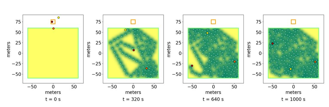
So a second layer sits above it. The field is partitioned into cells, each with a representative variance, and a Markov decision process rewards cells that are both uncertain and nearby — σ²/distance. Dynamic programming produces an ordered list of cells for each robot, and the QP takes the next waypoint as its nominal input while still enforcing its constraints.

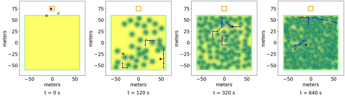
The two layers cover each other’s weaknesses, and the paper is explicit that neither works alone: planning by itself samples only at representative points and certifies nothing about mission efficiency, while the QP by itself gets stuck.

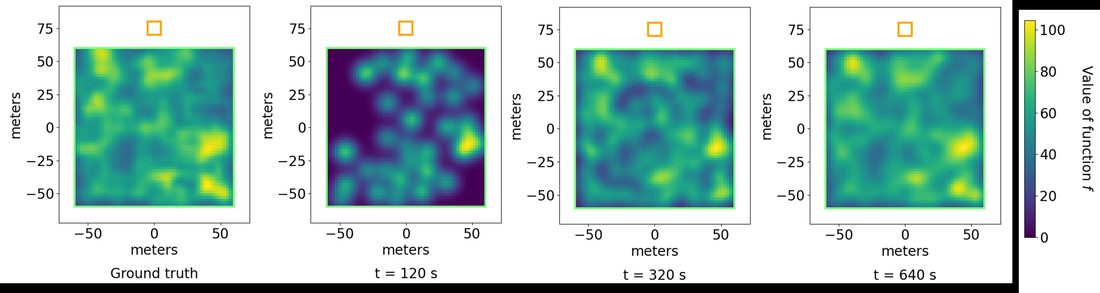
Both controllers eventually violate the decay-rate constraint — sensor noise means the variance can never reach zero. What separates them is the mean squared error at rest: near zero for the hierarchical controller, visibly nonzero for the constraint-based one.

Work with Masaya Suenaga and Kuniaki Uto at the Hatanaka Laboratory, presented at the European Control Conference 2025 in Thessaloniki.